
The DRTxECM interface is in English. Every button and field name below is quoted verbatim from the program, so that you can follow along on screen. The overall workflow is a fixed seven-step sequence.
In the Import Data section on the left side of the main window, click Import and select a CSV or TXT file; the "EIS Data Import Preprocessing Panel (DRTxECM)" window then opens.
Different instruments (BioLogic, Autolab, Solartron, Gamry…) export different numbers of header rows and different column orders, and this window exists to handle those differences:
| Control | Purpose |
|---|---|
| Number of rows to skip | Specify how many rows to skip at the start of the file (instrument header, comments, blank rows) |
| Toggle Column 3 (Z'') Sign (* -1) | Multiply the third column (the imaginary part) by −1. Some instruments store Z'' as positive, which turns the Nyquist plot upside down; use this button to correct it |
| Confirm and Import | Confirm and import |
After importing, the data appear in the main window and an EIS plot is shown at the top of the screen.
The data-parsing logic lives in DataImportPreprocessor; if your file format is unusual,
the source is in pyDRTtools/extensions.py.
The menu bar has a separate action, Clean Noise Data (shortcut Ctrl+D). Clicking it opens the "EIS Interactive Data Cleaning Interface".
On the Nyquist plot, click directly on the data points you want to remove to delete them; there is no need to go back and edit the source file.
| Button | Purpose |
|---|---|
| ↩ Undo Last Deletion | Undo the last deletion |
| Reset All Changes | Restore all deleted points |
| Apply Cleaning and Return | Apply and return to the main window |
The window shows Current active data points: — the number of remaining points — live,
so that you can see how many points you have deleted.
Once cleaning is finished, the program resamples the data onto a uniform logarithmic frequency grid using PCHIP monotone interpolation. The numerical DRT method requires a uniform frequency grid, so this step is not a plain deletion of data: it resamples at the same time. If your data are already uniform and clean, you may skip this step.
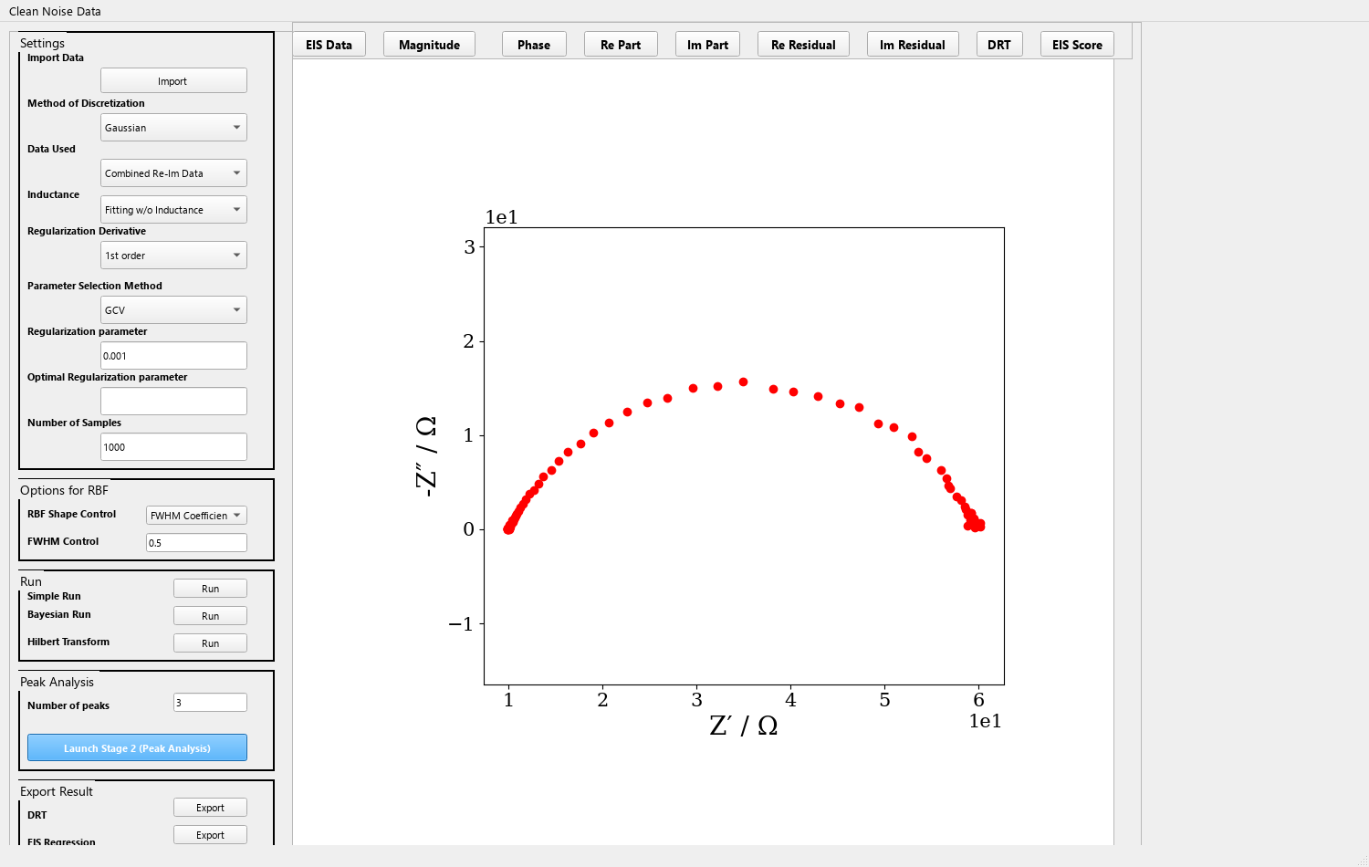
The left side of the main window holds the DRT settings; the upper right shows the plots and the lower right the run buttons. The settings are as follows:
| Field | Options | Description |
|---|---|---|
| Method of Discretization | Gaussian (default), C2 Matern, C4 Matern, C6 Matern, Inverse Quadratic, Inverse Quadric, Cauchy, PWL | The basis functions (radial basis) used to discretize γ(τ). Gaussian is the most common starting point; PWL is piecewise linear |
| Data Used | Combined Re-Im Data (default), Re Data, Im Data | Whether the fit uses the real part, the imaginary part, or both. Both are used by default |
| Inductance | Fitting w/o Inductance (default), Fitting with Inductance, Discard Inductive Data | Whether the inductive behavior at the high-frequency end is fitted along with the rest, ignored, or whether the data in the inductive region are simply discarded |
| Regularization Derivative | 1st order (default), 2nd order | The order of the derivative in the regularization term, which controls the smoothness of γ(τ) |
| Parameter Selection Method | custom, GCV (the default at program start), mGCV, rGCV, LC, kf, re-im | How the regularization parameter λ is determined. With custom it is set manually in the field below |
| Regularization parameter | default 0.001 |
The manual value of λ (used only in custom mode) |
| Optimal Regularization parameter | read-only | The λ selected automatically by the program; it is displayed here after a run |
| Number of Samples | default 1000 |
Number of samples for the Bayesian-related methods (Bayesian / BHT) |
| RBF Shape Control | FWHM Coefficient (default), Shape Factor | How the width of the basis functions is determined |
| FWHM Control | default 0.5 |
The width coefficient of the basis functions. Larger = smoother; smaller = higher resolution but more prone to oscillation |
Once configured, three DRT algorithms can be run from the lower right, each with its own Run button:
| Button | Method |
|---|---|
| Simple Run | Ridge regression / Tikhonov regularization. The fastest; use this first in ordinary cases |
| Bayesian Run | Bayesian regularization, estimating the noise and regularization hyperparameters jointly |
| Hilbert Transform | BHT (Bayesian Hilbert Transform), a variant that makes use of the Kramers-Kronig relations |
The right side of the main window has a row of display buttons that switch between plots:
| Button | Plot contents |
|---|---|
| EIS Data | Nyquist plot of the raw EIS data |
| Magnitude | Impedance magnitude |Z| of the Bode plot |
| Phase | Phase angle of the Bode plot |
| Re Part | Real part versus frequency |
| Im Part | Imaginary part versus frequency |
| Re Residual | Real-part residual (experimental value − fitted value) |
| Im Residual | Imaginary-part residual |
| DRT | The γ(τ) distribution, that is, the target of the decomposition in the next step |
| EIS Score | The goodness-of-fit score of each method, used to compare different settings |
A tip for judging quality: the residuals should scatter randomly around zero and should not curve systematically. If the residuals show clear structure, it usually means that the number of peaks is insufficient, that the regularization parameter λ is unsuitable, or that the high-frequency inductance has not been handled properly.
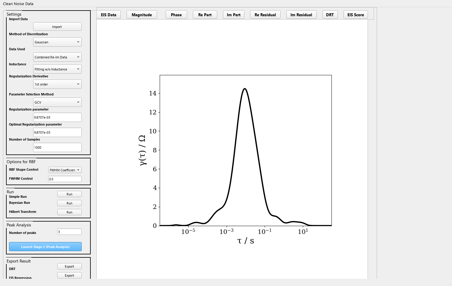
In the Peak deconvolution section, enter the Number of peaks (default 3),
then click the blue Launch Stage 2 (Peak Analysis) button to open the
"Stage 2: DRT Peak Fitting (DRTxECM)" window.
This window performs a multi-Gaussian peak fit on the γ(τ) obtained in the previous step, splitting the continuous distribution into a number of discrete peaks:
| Button | Purpose |
|---|---|
| View Initial Guess (Plot Guess) | Show the initial guess generated automatically by the program first, without optimizing |
| Execute Gaussian Fit | Run the multi-Gaussian fit |
| Export Stage 2 Decomposition Report (.csv) | Export the decomposition report: the parameters of each peak, together with the sampled points of each peak's fitted curve |
| Export to Stage 3 (CPE Fine-Tuning) | Convert the peak parameters into initial R//CPE values and open the third stage |
Each peak has three fields, each with its own check box:
| Field | Meaning |
|---|---|
amp | Peak amplitude Ai |
cen | Peak center position μi (in ln τ) |
wid | Peak width σi (default 0.8) |
Checked = lock that parameter (it is held fixed and given no room to vary); unchecked = let the fit adjust it freely. If you are confident about the physical location of a given peak, locking it lets the other peaks converge more stably.
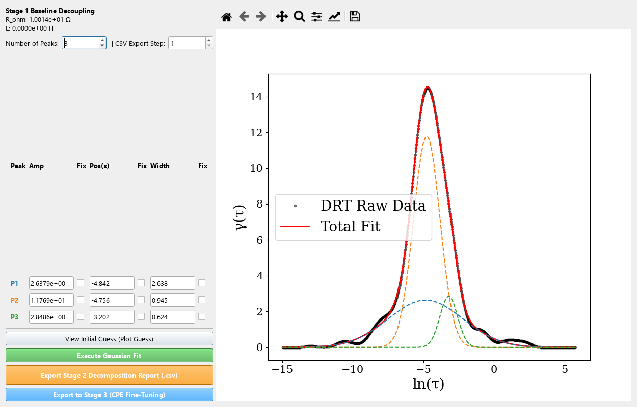
amp, position cen and width wid; on the right the
black dots are the raw DRT data, the red line is the sum of the three peaks, and the coloured
dashed curves are the individual peaks. The top left also shows the R_ohm resolved in
Stage 1 (10.014 Ω for this sample).
Clicking Export to Stage 3 (CPE Fine-Tuning) opens the "Stage 3: ECM Fine-Tune Panel (DRTxECM)".
The program performs the following conversion automatically (each Gaussian peak corresponds to one R//CPE branch):
In other words, the DRT peaks are not merely a visual decomposition: they directly provide a physically reasonable starting point. This is one of the greatest advantages of DRTxECM over general-purpose circuit-fitting tools.
The columns of the table on the left are Element | Freedom | Value | Error | Error%:
| Element | Corresponding circuit element |
|---|---|
R_ohm | The series ohmic resistance R0 (high-frequency intercept) |
L_ind | The series inductance L |
R_i | Resistance of the i-th branch |
Q_i | CPE parameter Q of the i-th branch |
n_i | The CPE phase angle α of the i-th branch (0.2 to 1.0 or 1.05) |
The Freedom column determines how free each parameter is during optimization. Different element types offer different modes (these are the exact strings shown in the interface):
| Element | Available modes | Allowed range |
|---|---|---|
R_i, Q_i |
Free, Free +-5%, Free +-10%, Fixed |
Free: 0 to ∞; Free +-5% / Free +-10%: ±5% / ±10% of the current value; Fixed: locked |
n_i (that is, α) |
Free, <= 1, Fixed |
<= 1: 0.2 to 1.0; Free: 0.2 to 1.05; Fixed: locked |
L_ind |
Free, Fixed |
Free: −∞ to ∞; Fixed: locked |
R, Q and L all default to Fixed, and α defaults to <= 1,
so on first entering Stage 3 only the three α values can be optimized.
The recommended order is: let the α values converge first, then release R and Q one at a time.
In the formal literature the theoretical upper bound for the CPE α is 1 (an ideal capacitor).
The program also offers a mode that allows up to 1.05, in order to absorb measurement error and
deviations in the equivalent series resistance, so that the fit does not get stuck on a hard boundary.
If you need the α in your report to conform strictly to the physical definition, use <= 1.
The bottom of the window shows Complex Impedance RMSE, which is updated after Fitting
to the RMSE value with units.
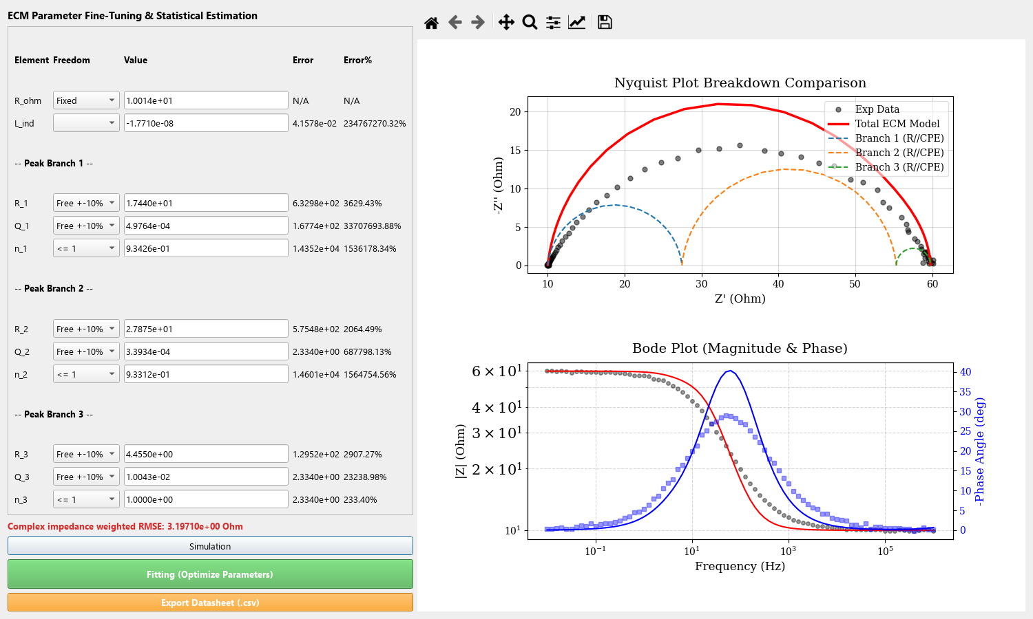
Free +-10% and α set to
<= 1. Note the Error% column: this example fits a single ZARC semicircle
with three branches, which over-parameterizes the data, so the standard errors are large.
In practice the number of peaks should match the actual peaks in the DRT curve rather than being
increased just to lower the RMSE.
| Location | Button | What is exported |
|---|---|---|
| Main window, Export section | DRT → Export | The γ(τ) result of the DRT (frequency, τ, γ) |
| Main window, Export section | EIS Regression → Export | The fitted EIS values and the residuals |
| Main window, Export section | Figure → Save | The figure currently displayed |
| Stage 2 | Export Stage 2 Decomposition Report (.csv) | The peak parameters and the decomposition curve of each peak |
| Stage 3 | Export Datasheet (.csv) | The circuit parameters, standard errors, and the combined report after fitting |
The warning No EIS data loaded! appears. Click Import to load data first.
This is usually under-regularization (λ too small) or an FWHM Control that is too small. You can: leave Parameter Selection Method on GCV so that the program selects λ automatically; increase FWHM Control; or switch to Bayesian Run.
The common cause is initial values that lie too far from the true values. The recommended order is:
use Stage 2 first to obtain a good initial guess → in Stage 3, release the parameters one at a
time rather than setting them all to free at once. In practice, release R and Q first
and release α once they have converged; this is much more stable.
This means that the optimum lies on a boundary. If it sticks at 1.0, the branch may in fact be close to an ideal capacitor, or the data quality may not support a free fit of α; if it sticks at 0.2, the frequency range of that branch is usually too narrow or it has too few points. You can check the branch's coverage in the Nyquist plot.
N/A or <15%
The uncertainty is estimated from the inverse Hessian matrix. If the Hessian cannot be obtained or is
unstable, the program falls back to displaying N/A; in some cases it shows
<15% instead, as a rough upper bound on the relative error. This is not an error, but
it does mean that the standard errors for that parameter set should be treated with caution.
The multi-Gaussian fit iterates at most 10000 times. The more peaks there are, the slower it is. Start with 2 to 4 peaks and increase the number once you have confirmed the shape of γ(τ).